Getting started with matplotlib

Bear with me; this is my first blog post.

I want to write about something that I care about. I care about software and I care about science. More importantly, I care about how these two interact and how software can help the scientific community. Presentation of science to the public in an understandable fashion is difficult. It’s always hard to gauge at what level a scientist should pitch their presentation, and that’s where pictures come in handy.

Most people abosrb information best visually. Auditory and kinematic learners also exist, but most people are visual learners. To that end, I decided to write about matplotlib, a plotting library written in Python. This should be fairly introductory.

Installing

For some reason, installing python packages is notoriously hard if you’re not exposed to the various different approaches already out there. I’m not going to go through all of them. Instead, I recommend you install matplotlib through your operating system’s package manager. If you’re on Ubuntu, it’s aptitude. If you’re on RHEL, it’s yum. If you’re on OS X, you don’t have a package manager by default and you should install one. I recommend macports, but others speak volumes about homebrew.

Personally, I like to install software from source by hand. If you’re scared of doing it you should give it a try. It’s super educational. I will go through the installation from source procedure on a Mac in another blog post, since I don’t want to bloat this one. In what remains, I’ll assume you have it installed.

To check you have installed matplotlib correctly, you can execute the following in a terminal:

$ python -c "import matplotlib"
$ echo $?
0

The command echo $? just prints out the exit status of the previous command. If you get a 0 then the previous command was successful. If you get a 1, or anything nonzero, then matplotlib is not installed correctly.

Your first plot

Now that matplotlib is installed correctly, you can create your first plot.

From now on, I’ll be using the IPython prompt, but you don’t need that to along. All the commands are the same and will work in the regular python prompt.

First, we boot up the ipython console:

$ ipython
Python 2.7.3 (default, Nov 29 2012, 11:01:29)
Type "copyright", "credits" or "license" for more information.

IPython 0.13.2 -- An enhanced Interactive Python.
?         -> Introduction and overview of IPython's features.
%quickref -> Quick reference.
help      -> Python's own help system.
object?   -> Details about 'object', use 'object??' for extra details.

In [1]: 

Now we import pyplot, a set of convenience methods that interface well with matplotlib’s internals:

In [1]: import matplotlib.pyplot as plt

Next, we create a Figure object:

In [2]: fig = plt.figure()

The Figure is the object that holds the axes, which we create now:

In [3]: ax = fig.add_subplot(1, 1, 1)

The Axes [1] object is where most of the magic happens. This is the object you will interface with the most to do all of your plotting. Here is a simple plotting command that creates a line plot:

In [4]: ax.plot([1, 2, 3], [1, 4, 9])
Out[4]: [<matplotlib.lines.Line2D at 0x10860ad50>]

The plot function takes a list of x-coordinates and a list of y-coordinates and returns a list of objects called Line2D objects. A Line2D object is a matplotlib object that represents the lines in the figure that join the coordinates together. We will explore Line2D objects, and other objects, in a different post. For now, just take it for granted that ax.plot connects the passed coordinates with lines to create a line plot. We can save the figure with the following:

In [5]: fig.savefig('plot.pdf')

This will save the figure in pdf format. Open it and take a look. It should look a little like this:

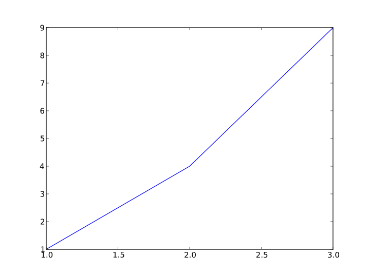
There are lots of file types that matplotlib supports. The ones I use most commonly are pdf and png. In fact, the image above is an svg file. It is common in the scientific community to produce scalable vector graphics, and matplotlib allows this. It also supports ps and eps. For a full list of supported file types see here.

[1] It’s actually an AxesSubplot object, not an Axes object. An AxesSubplot is just an Axes object with some extra functions to allow manipulation of its position within a Figure. The reason for this is that there may be more than one set of axes in a figure.

Another example

You can stop here, or you can follow along with a more complicated line plot using numpy, a high performance python library for dealing with array objects. Carrying on from within the same ipython session:

In [6]: ax.cla()

This clears the axes of the old plot ready to plot something new.

In [7]: import numpy as np

Here we import numpy so we can use it below:

In [8]: x = np.linspace(0, 5, num=1000, endpoint=True)

This creates an array, x, of 1000 equally spaced points between 0 and 1, inclusive.

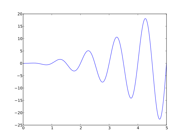
In [9]: y = x * x * np.sin(2.0 * np.pi * x)

This line takes advantage of some of numpy’s machinery. The multiplication of numpy arrays is done component-wise.

In [10]: ax.plot(x, y)
Out[10]: [<matplotlib.lines.Line2D at 0x108a728d0>]

Again, we pass in the x- and y-coordinates to plot. This draws lines between the passed coordinates. Go ahead and save your creation. It should look something like this: